disturbances_2013_moja#
You can find instructions to open a geoTIFF file here. Instructions on how to download and install Rasterio and GDAL(not necessary for linux) are included too.
In addition to that, we also need to install matplotlib and Shapely in order to clip the raster.
To install matplotlib and Shapely, run the commands :
pip install matplotlib
pip install shapely
Import the required libraries
import rasterio as rst
from rasterio.plot import show
import matplotlib.pyplot as plt
import numpy as np
Store the geoTIFF file in a variable, use the rs.open() and show() functions to open view the image in the next cell.
We can also perform different operations using raster objects: the number of bands, the image resolution, CRS value, no-data value, number of raster bands, etc.
disturbances13 = r'disturbances_2013_moja.tiff'
img = rst.open(disturbances13)
show(img)
#No. of bands
print(img.count)

#Image resolution
print(img.height, img.width)

# CRS
print(img.crs)

# No-data
print(img.nodata)

1
4000 4000
EPSG:4326
255.0
The image has a lot of padding around the area of interest, hence we need to clip the raster.
from rasterio.features import dataset_features
Finding geometry for a mask
dataset_features yields GeoJSON-like feature dictionaries for shapes found in the given band
Using this, we get the bounding box from all shapes in the output
geom_gen = dataset_features(img, bidx=1)
bboxes = [geom['bbox'] for geom in geom_gen]
bboxes
[[-105.84875, 54.48625, -105.8485, 54.4865],
 [-105.86425, 54.47975, -105.84875, 54.48625],
 [-105.861, 54.4675, -105.84025, 54.476],
 [-105.86125, 54.46725, -105.861, 54.4675]]
Next, we assign the extremums from the bounding box to different variables
left   = min([bbox[0] for bbox in bboxes])
bottom = min([bbox[1] for bbox in bboxes])
right  = max([bbox[2] for bbox in bboxes])
top    = max([bbox[3] for bbox in bboxes])
Create a Polygon geometry for the mask
from shapely.geometry import box

# create a POLYGON geometry for the mask
geom = box(left, bottom, right, top)
geom.wkt
'POLYGON ((-105.84025 54.46725, -105.84025 54.4865, -105.86425 54.4865, -105.86425 54.46725, -105.84025 54.46725))'
Creating the mask
from rasterio.mask import mask
Assigning the data for the clipped image
out_image, out_transform = mask(img, [geom], crop=True, pad=True)
out_meta = img.meta
out_meta.update({"driver": "GTiff",
                 "height": out_image.shape[1],
                 "width": out_image.shape[2],
                 "transform": out_transform})

with rst.open(r'disturbances_2013_moja_masked.tiff', 'w', **out_meta) as dest:
    dest.write(out_image)
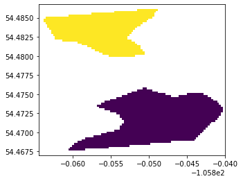
View the clipped raster
fp_result = r'disturbances_2013_moja_masked.tiff'
result = rst.open(fp_result)
show(result)
<AxesSubplot:>
View JSON data parsed from disturbances_2013_moja
import json
with open("disturbances_2013_moja.json") as f:
      data = json.load(f)
data
{'layer_type': 'GridLayer',
 'layer_data': 'Byte',
 'nodata': 255,
 'tileLatSize': 1.0,
 'tileLonSize': 1.0,
 'blockLatSize': 0.1,
 'blockLonSize': 0.1,
 'cellLatSize': 0.00025,
 'cellLonSize': 0.00025,
 'attributes': {'1': {'year': 2013,
   'disturbance_type': 'Mountain pine beetle — Very severe impact',
   'transition': 1},
  '2': {'year': 2013, 'disturbance_type': 'Wildfire', 'transition': 1}}}